Deep Learning Research Review Week 2: Reinforcement Learning

This is the 2^nd installment of a new series called Deep Learning Research Review. Every couple weeks or so, I’ll be summarizing and explaining research papers in specific subfields of deep learning. This week focuses on Reinforcement Learning. Last time was Generative Adversarial Networks ICYMI

Introduction to Reinforcement Learning

3 Categories of Machine Learning

Before getting into the papers, let’s first talk about what reinforcement learning is. The field of machine learning can be separated into 3 main categories.

Supervised Learning
Unsupervised Learning
Reinforcement Learning

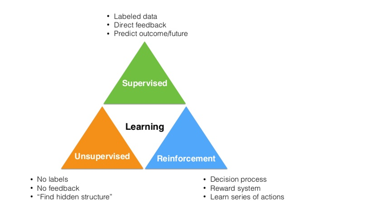
The first category, supervised learning, is the one you may be most familiar with. It relies on the idea of creating a function or model based on a set of training data, which contains inputs and their corresponding labels. Convolutional Neural Networks are a great example of this, as the images are the inputs and the outputs are the classifications of the images (dog, cat, etc).

Unsupervised learning seeks to find some sort of structure within data through methods of cluster analysis. One of the most well-known ML clustering algorithms, K-Means, is an example of unsupervised learning.

Reinforcement learning is the task of learning what actions to take, given a certain situation/environment, so as to maximize a reward signal. The interesting difference between supervised and reinforcement learning is that this reward signal simply tells you whether the action (or input) that the agent takes is good or bad. It doesn’t tell you anything about what the best action is. Contrast this to CNNs where the corresponding label for each image input is a definite instruction of what the output should be for each input. Another unique component of RL is that an agent’s actions will affect the subsequent data it receives. For example, an agent’s action of moving left instead of right means that the agent will receive different input from the environment at the next time step. Let’s look at an example to start off.

The RL Problem

So, let’s first think about what have in a reinforcement learning problem. Let’s imagine a tiny robot in a small room. We haven’t programmed this robot to move or walk or take any action. It’s just standing there. This robot is our agent.

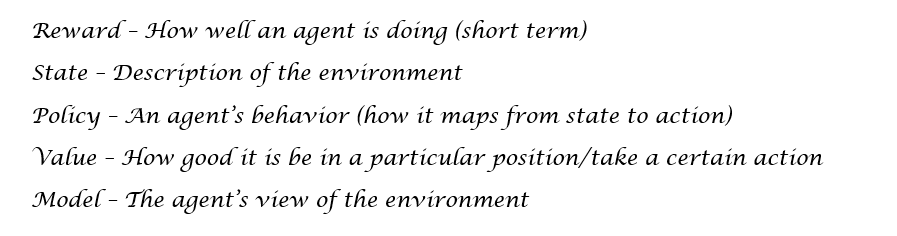
Like we mentioned before, reinforcement learning is all about trying to understand the optimal way of making decisions/actions so that we maximize some reward R. This reward is a feedback signal that just indicates how well the agent is doing at a given time step. The action A that an agent takes at every time step is a function of both the reward (signal telling the agent how well it’s currently doing) and the state S, which is a description of the environment the agent is in. The mapping from environment states to actions is called our policy P. The policy basically defines the agent’s way of behaving at a certain time, given a certain situation. Now, we also have a value function V which is a measure of how good each position is. This is different from the reward in that the reward signal indicates what is good in the immediate sense, while the value function is more indicative of how good it is to be in this state/position in the long run. Finally, we also have a model M which is the agent’s representation of the environment. This is the agent’s model of how it thinks that the environment is going to behave.

Markov Decision Process

So, let’s now think back to our robot (the agent) in the small room. Our reward function is dependent on what we want the agent to accomplish. Let’s say that we want it to move to one of the corners of the room where it will receive a reward. The robot will get a +25 when it reaches this point, and will get a -1 for every time step it takes to get there. We basically want the robot to get the corner as fast as possible. The actions the agent can take are moving north, south, east, or west. The agent’s policy can be a simple one, where the behavior is that the agent will always move to the location with the higher value function. Makes sense right? A position with a high value function = good to be in this position (with regards to long term reward).

Now, this whole RL environment can be described with a Markov Decision Process. For those that haven’t heard the term before, an MDP is a framework for modeling an agent’s decision making. It contains a finite set of states (and value functions for those states), a finite set of actions, a policy, and a reward function. Our value function can be split into 2 terms.

State-value function V: The expected return from being in a state S and following a policy π. This return is calculated by looking at summation of the reward at each future time step (The gamma refers to a constant discount factor, which means that the reward at time step 10 is weighted a little less than the reward at time step 1).

Action-value function Q: The expected return from being in a state S, following a policy π, and taking an action a (Equation will be same as above except that we have an additional condition that A_t = a).

Now that we have all the components, what do we do with this MDP? Well, we want to solve it, of course. By solving an MDP, you’ll be able to find the optimal behavior (policy) that maximizes the amount of reward the agent can expect to get from any state in the environment.

Solving the MDP

We can solve an MDP and get the optimum policy through the use of dynamic programming and specifically through the use of policy iteration (there is another technique called value iteration, but won’t go into that right now). The idea is that we take some initial policy π₁ and evaluate the state value function for that policy. The way we do this is through the Bellman expectation equation.

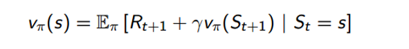
This equation basically says that our value function, given that we’re following policy π, can be decomposed into the expected return sum of the immediate reward R_t+1 and the value function of the successor state S_t+1. If you think about it closely, this is equivalent to the value function definition we used in the previous section. Using this equation is our policy evaluation component. In order to get a better policy, we use a policy improvement step where we simply act greedily with respect to the value function. In other words, the agent takes the action that maximizes value.

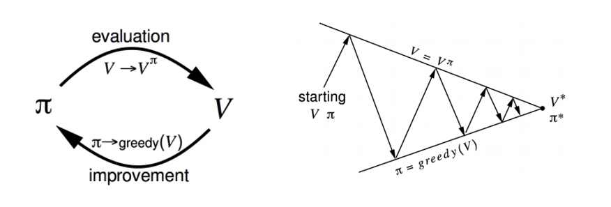
Now, in order to get the optimal policy, we repeat these 2 steps, one after the other, until we converge to optimal policy π^*.

When You’re Not Given an MDP

Policy iteration is great and all, but it only works when we have a given MDP. The MDP essentially tells you how the environment works, which realistically is not going to be given in real world scenarios. When not given an MDP, we use model free methods that go directly from the experience/interactions of the agents and the environment to the value functions and policies. We’re going to be doing the same steps of policy evaluation and policy improvement, just without the information given by the MDP.

The way we do this is instead of improving our policy by optimizing over the state value function, we’re going to optimize over the action value function Q. Remember how we decomposed the state value function into the sum of immediate reward and value function of the successor state? Well, we can do the same with our Q function.

Now, we’re going to go through the same process of policy evaluation and policy improvement, except we replace our state value function V with our action value function Q. Now, I’m going to skip over the details of what changes with the evaluation/improvement steps. To understand MDP free evaluation and improvement methods, topics such as Monte Carlo Learning, Temporal Difference Learning, and SARSA would require whole blogs just themselves (If you are interested, though, please take a listen to David Silver’s Lecture 4 and Lecture 5). Right now, however, I’m going to jump ahead to value function approximation and the methods discussed in the AlphaGo and Atari Papers, and hopefully that should give a taste of modern RL techniques. The main takeaway is that we want to find the optimal policy π^* that maximizes our action value function Q.

Value Function Approximation

So, if you think about everything we’ve learned up until this point, we’ve treated our problem in a relatively simplistic way. Look at the above Q equation. We’re taking in a specific state S and action A, and then computing a number that basically tells us what the expected return is. Now let’s imagine that our agent moves 1 millimeter to the right. This means we have a whole new state S’, and now we’re going to have to compute a Q value for that. In real world RL problems, there are millions and millions of states so it’s important that our value functions understand generalization in that we don’t have to store a completely separate value function for every possible state. The solution is to use a Q value function approximation that is able to generalize to unknown states.

So, what we want is some function, let’s call is Qhat, that gives a rough approximation of the Q value given some state S and some action A.

This function is going to take in S, A, and a good old weight vector W (Once you see that W, you already know we’re bringing in some gradient descent ). It is going to compute the dot product between x (which is just a feature vector that represents S and A) and W. The way we’re going to improve this function is by calculating the loss between the true Q value (let’s just assume that it’s given to us for now) and the output of the approximate function.

After we compute the loss, we use gradient descent to find the minimum value, at which point we will have our optimal W vector. This idea of function approximation is going to be very key when taking a look at the papers a little later.

Just One More Thing

Before getting to the papers, just wanted to touch on one last thing. An interesting discussion with the topic of reinforcement learning is that of exploration vs exploitation. Exploitation is the agent’s process of taking what it already knows, and then making the actions that it knows will produce the maximum reward. This sounds great, right? The agent will always be making the best action based on its current knowledge. However, there is a key phrase in that statement. Current knowledge. If the agent hasn’t explored enough of the state space, it can’t possibly know whether it is really taking the best possible action. This idea of taking actions with the main purpose of exploring the state space is called exploration.

This idea can be easily related to a real world example. Let’s say you have a choice of what restaurant to eat at tonight. You (acting as the agent) know that you like Mexican food, so in RL terms, going to a Mexican restaurant will be the action that maximizes your reward, or happiness/satisfaction in this case. However, there is also a choice of Italian food, which you’ve never had before. There’s a possibility that it could be better than Mexican food, or could be a lot worse. This tradeoff between whether to exploit an agent’s past knowledge vs trying something new in hope of discovering a greater reward is one of the major challenges in reinforcement learning (and in our daily lives tbh).

Other Resources for Learning RL

Phew. That was a lot of info. By no means, however, was that a comprehensive overview of the field. If you’d like a more in-depth overview of RL, I’d strongly recommend these resources.

David Silver (from Deepmind) Reinforcement Learning Video Lectures
- My personal notes from the RL course
Sutton and Barto’s Reinforcement Learning Textbook (This is really the holy grail if you are determined to learn the ins and outs of this subfield)
Andrej Karpathy’s Blog Post on RL (Start with this one if you want to ease into RL and want to see a really well done practical example)
UC Berkeley CS 188 Lectures 8-11
Open AI Gym: When you feel comfortable with RL, try creating your own agents with this reinforcement learning toolkit that Open AI created

DQN For Reinforcement Learning (RL With Atari Games)

Introduction

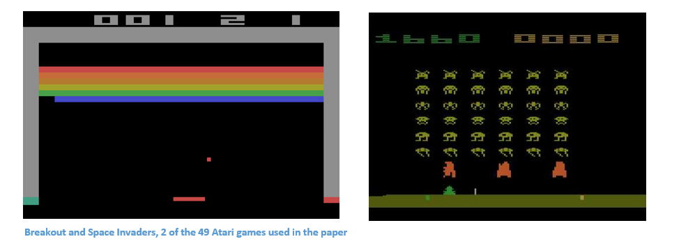
This paper was published by Google Deepmind in February of 2015 and graced the cover of Nature, a world famous weekly journal of science. This was one of the first successful attempts at combining deep neural networks with reinforcement learning (This was Deepmind’s original paper). The paper showed that their system was able to play Atari games at a level comparable to professional game testers across a set of 49 games. Let’s take a look at how they did it.

Approach

Okay, so remember where we left off in the intro tutorial at the beginning of the post? We had just described the main goal of having to optimize our action value function Q. The folks at Deepmind approached this task through a Deep Q-Network, or a DQN. This network is able to come up with successful policies that optimize Q, all from inputs in the form of pixels from the game screen and the current score.

Network Architecture

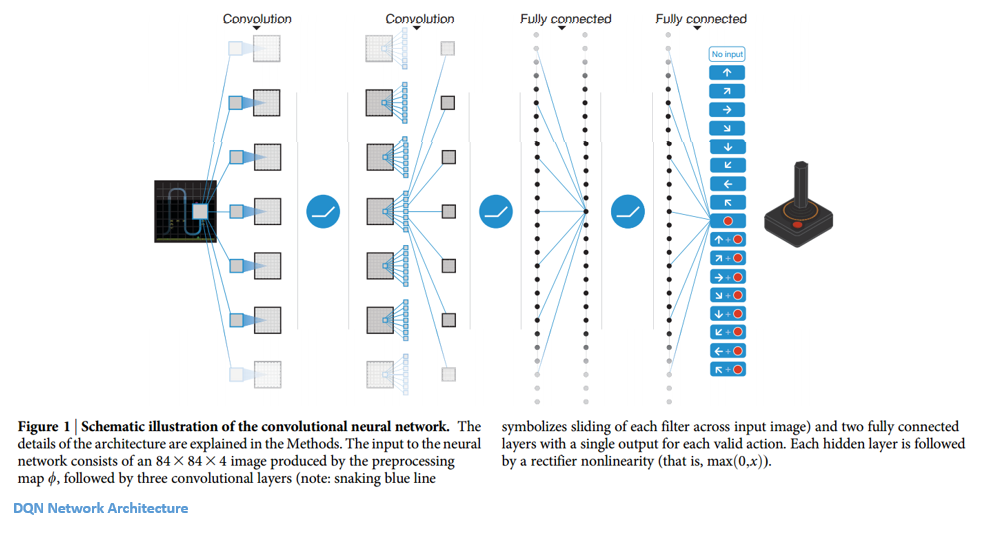
Let’s take a closer look at what inputs this DQN will have. Consider the game of Breakout, and take 4 of the most recent frames in the current game. Each of these frame originally starts as a 210 x 160 x 3 image (because width and height are 210 and 160 pixels and it is a color image). Then, some preprocessing takes place where the frames are scaled to 84 x 84 (not extremely important to know how this is done, but check page 6 for details). So, now we have an 84 x 84 x 4 input volume. This volume is going to get plugged into a convolutional neural network (tutorial) where it will go through a series of conv and ReLU layers. The output of the network is an 18 dimensional vector where each number is the Q-value for each possible action the user can take (move up, down, left, etc).

Okay, so let’s take a step back for a second and figure out how we’re going to train this network so that It will predict accurate Q-values. Let’s first remember what we’re trying to optimize.

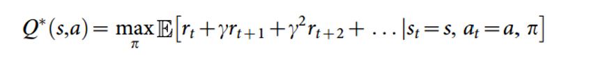
This is the same form as the Q function we saw earlier, except this one represents Q* which is the max over all Q’s. Let’s examine how we’re going to get this Q*. Now, remember we just want an approximation for Q*, which is where our function approximators are going to come in (our Qhats). Just keep that thought in your head while we switch gears a little.

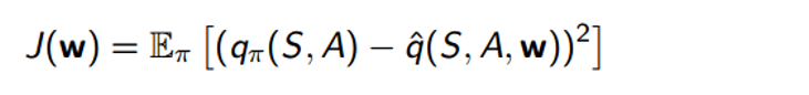
In order to find the best policy, we want to frame some sort of supervised learning problem where the predicted Q function is compared to some expected one, and then is adjusted in the correct direction. In order to do that, we need a set of training examples. In our case, we are going to have to create a set of experiences that store the agent’s state, action, reward, and next state for every time step. Let’s formalize that a bit more. We have a replay memory D which contains (s_t, a_t,r_t,s_t+1) for a bunch of different time steps. This dataset gets built over time, as the agent interacts more with the environment. Now, we’re going a take a random batch of this data (let’s say data for 64 time steps), compute the loss function for each of them, and then follow the gradient to improve our Q function approximation.

So, as you can see, the loss function wants to optimize the mean squared error (MSE) between the Q network function approximation (Q(s,a,theta)) and the Q learning targets. Let me quickly explain those. This Q learning target is the reward r plus the maximum Q value (in the next time step) that you can get from some action a’.

Once the loss function is computed, the derivatives are taken w.r.t the theta values (or the w vector). These values are then updated so as to minimize the loss function.

Conclusion

One of my favorite parts about the paper is this visualization it gives of the value function during certain points of the game.

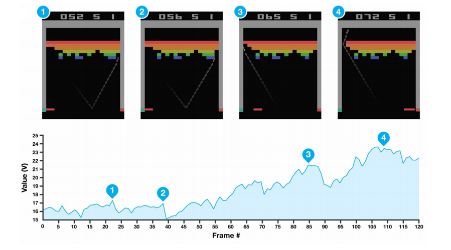
As you remember, the value function is basically a metric for measuring “how good it is to be in a particular situation”. If you look at #4, you can see, based on the trajectory of the ball and the location of the bricks, that we’re in for a lot of points and the high value function is quite representative of that.

All 49 Atari games used the same network architecture, algorithm, and hyperparameters which is an impressive testament to the robustness of such an approach to reinforcement learning. The combination of deep networks and traditional reinforcement learning strategies, like Q learning, proved to be a great breakthrough in setting the stage for……

Mastering AlphaGo with RL

Introduction

4-1. That’s the record Deepmind’s RL agent had against one of the best Go players in the world, Lee Sedol. In case you didn’t know, Go is an abstract strategy game of capturing territory on a game board. It is considered to be one of the hardest games in the world for AI because of the incredible number of different game scenarios and moves. The paper begins with a comparison of Go and common board games like chess and checkers. While those can be attacked with variations of tree search algorithms, Go is a totally different animal because there are about 250¹⁵⁰ different sequences of moves in a game. It’s clear that reinforcement learning was needed, so let’s look into how AlphaGo managed to beat the odds.

Approach

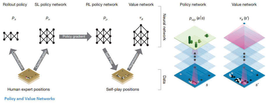
The basis behind AlphaGo are the ideas of evaluation and selection. With any reinforcement learning problem (especially with a board game), you need a way of evaluating the environment, or the current board position. This is going to be our value network. You then need a way of selecting an action to take through a policy network. We’ve definitely had experience with both of these terms, value and policy.

Network Architecture

Let’s look at what inputs both of these networks are going to take. The board position is passed in as a 19 x 19 image that goes through a series of conv layers to construct a good representation of the current state. So let’s first look at our SL (Supervised Learning) policy network. This network is going to take in the image as input and then output a probability distribution over all of the legal actions the agent can take. This network is pretrained (before the actual game) on 30 million different Go board positions. Each of these board positions is labeled with what an expert move would be in that situation. The team also trained a smaller, but faster rollout policy network.

Now, CNNs can only do so much to predict the correct move you should take, given a representation of the current board. That’s when reinforcement learning comes in. We’re going to improve this policy network through a process called policy gradients. Remember how in the last paper, we wanted to optimize our action value function Q? Well now, we’re going straight to optimizing our policy (Policy gradients take a while to explain but David Silver does a good job in Lecture 7). From a high level, the policy is improved by simulating games between the current policy network and a previous iteration of the network. The reward signal is +1 for winning the game, -1 for losing, and so we can improve the network through the normal gradient descent.

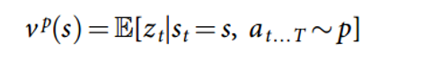
Okay, so now we have a pretty good network that tells us the best action to play. The next step is having a value network that predicts the outcome a game which is at board position S and where both players are using policy P.

In order to get the optimal V*, we’ll use our good old function approximators with weights W. The weights are trained by the value network which are conditioned on state, outcome pairs (similar to what we saw in the last paper).

Now that we have these main two networks, our final step is to use a Monte Carlo Tree Search to put everything together. The basic idea behind MCTS is that it selects the best actions through lookahead search where each edge in the tree stores an action value Q, a visit count, and a prior probability. From that info, the MCTS algorithm will pick the best action A from the current state. This part of the system is a little less RL and more traditional AI so if you’d like more details, definitely check out the paper, which will do a much better job of summarizing.

Conclusion

A computer system just beat the world’s best player at one of the hardest board games ever. Who even needs a conclusion?

via GIPHY

Big thanks to David Silver for the equations and the excellent lecture course on RL

Dueces.

Sources

Written on November 16, 2016