This is the 3^rd installment of a new series called Deep Learning Research Review. Every couple weeks or so, I’ll be summarizing and explaining research papers in specific subfields of deep learning. This week focuses on applying deep learning to Natural Language Processing. The last post was Reinforcement Learning and the post before was Generative Adversarial Networks ICYMI

Introduction to Natural Language Processing

Introduction

                Natural language processing (NLP) is all about creating systems that process or “understand” language in order to perform certain tasks. These tasks could include

• Question Answering (What Siri, Alexa, and Cortana do)
• Sentiment Analysis (Determining whether a sentence has a positive or negative connotation)
• Image to Text Mappings (Generating a caption for an input image)
• Machine Translation (Translating a paragraph of text to another language)
• Speech Recognition
• Part of Speech Tagging
• Name Entity Recognition

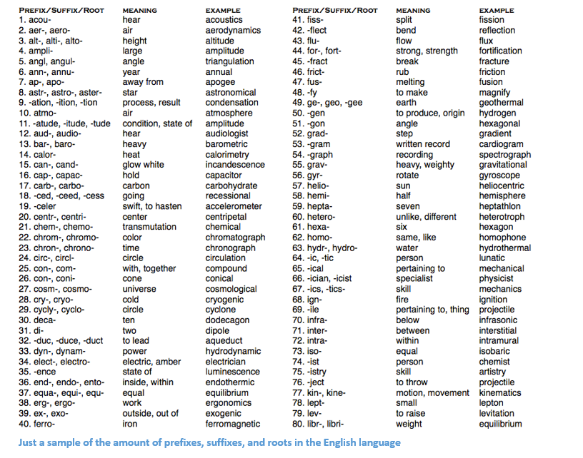
The traditional approach to NLP involved a lot of domain knowledge of linguistics itself. Understanding terms such as phonemes and morphemes were pretty standard as there are whole linguistic classes dedicated to their study. Let’s look at how traditional NLP would try to understand the following word.

Let’s say our goal is to gather some information about this word (characterize its sentiment, find its definition, etc). Using our domain knowledge of language, we can break up this word into 3 parts.

We understand that the prefix “un” indicates an opposing or opposite idea and we know that “ed” can specify the time period (past tense) of the word. By recognizing the meaning of the stem word “interest”, we can easily deduce the definition and sentiment of the whole word. Seems pretty simple right? However, when you consider all the different prefixes and suffixes in the English language, it would take a very skilled linguist to understand all the possible combinations and meanings.

How Deep Learning Fits In

                Deep learning, at its most basic level, is all about representation learning. With CNNs, we see the composition of different filters that are used to classify objects into categories. Here, we’re going to take a similar approach with creating representations of words through large datasets.

Overview of This Post

                This post will be structured in a way where we’ll go through the basic building blocks of building deep networks for NLP and then go into talking about some applications through recent research papers. It’ll feel normal to not exactly know why we’re using RNNs or why an LSTM is helpful, but hopefully by the end of the research papers, you’ll have a better sense of why deep learning techniques have helped NLP so much. 

Word Vectors

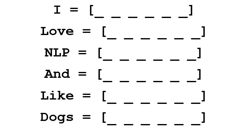
                Since deep learning loves math, we’re going to represent each word as a d-dimensional vector. Let’s use d = 6.

Now let’s think about how to fill in the values. We want the values to be filled in such a way that the vector somehow represents the word and its context, meaning, or semantics. One method is to create a coocurence matrix. Let’s say that we have the following sentence.

From this sentence, we want to create a word vector for each unique word.

A coocurence matrix is a matrix that contains the number of counts of each word appearing next to all the other words in the corpus (or training set). Let’s visualize this matrix.

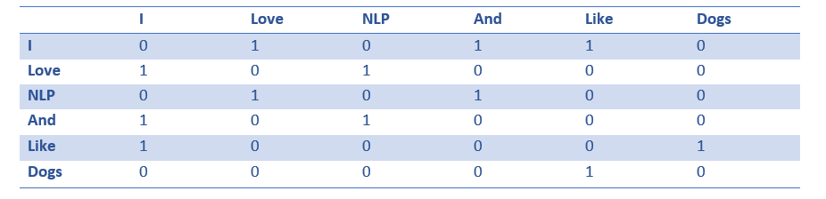
Extracting the rows from this matrix can give us a simple initialization of our word vectors.

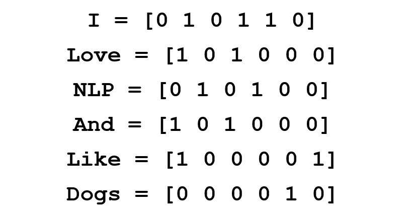
Notice that through this simple matrix, we’re able to gain pretty useful insights. For example, notice that the words ‘love’ and ‘like’ both contain 1’s for their counts with nouns (NLP and dogs). They also have 1’s for the count with “I”, thus indicating that the words must be some sort of verb. With a larger dataset than just one sentence, you can imagine that this similarity will become more clear as ‘like’, ‘love’, and other synonyms will begin to have similar word vectors, because of the fact that they are used in similar contexts.

Now, although this a great starting point, we notice that the dimensionality of each word will increase linearly with the size of the corpus. If we had a million words (not really a lot in NLP standards), we’d have a million by million sized matrix which would be extremely sparse (lots of 0’s). Definitely not the best in terms of storage efficiency. There have been numerous advancements in finding the most optimal ways to represent these word vectors. The most famous of which is Word2Vec.

Word2Vec

                The basic idea behind word vector initialization techniques is that we want to store as much information as we can in this word vector while still keeping the dimensionality at a manageable scale (25 – 1000 dimensions is ideal). Word2Vec operates on the idea that we want to predict the surrounding words of every word.  Let’s take our previous sentence “I love NLP and I like dogs”. We’re going to look at the first 3 words of this sentence. 3 is thus going to be our window size m.

Now, our goal is to take the center word, ‘love’, and predict the words that come before and after it. How do we do this? By maximizing/optimizing a function of course! Formally, our function seeks to maximize the log probability of any context word given the current center word.

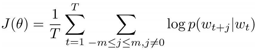
Let’s dig deeper into this. The above cost function is basically saying that we’re going to add the log probabilities of ‘I’ and ‘love’ as well as ‘NLP’ and ‘love’ (where ‘love’ is the center word in both cases). The variable T represents the number of training sentences. Let’s look closer at that log probability.

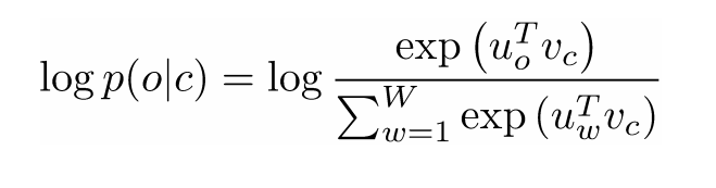
V_c is the word vector of the center word. Every word has two vector representations (U_o and U_w), one for when the word is used as the center word and one for when it’s used as the outer word. The vectors are trained with stochastic gradient descent. This is definitely one of the more confusing equations to understand, so if you’re still having trouble visualizing what’s happening, you can go here and here for additional resources.

One Sentence Summary: Word2Vec seeks to find vector representations of different words by maximizing the log probability of context words given a center word and modifying the vectors through SGD.

(Optional: The authors of the paper then go into more detail about how negative sampling and subsampling of frequent words can be used to get more precise word vectors. )

Arguably, the most interesting contribution of Word2Vec was the appearance of linear relationships between different word vectors. After training, the word vectors seemed to capture different grammatical and semantic concepts.

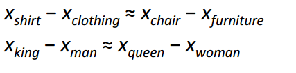
It’s pretty incredible how these linear relationships could be formed through a simple objective function and optimization technique.

Bonus: Another cool word vector initialization method: GloVe (Combines the ideas of coocurence matrices with Word2Vec)

Recurrent Neural Networks (RNNs)

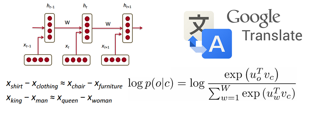
                Okay, so now that we have our word vectors, let’s see how they fit into recurrent neural networks. RNNs are the go-to for most NLP tasks today. The big advantage of the RNN is that it is able to effectively use data from previous time steps. This is what a small piece of an RNN looks like.

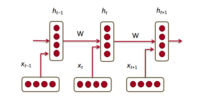
So, at the bottom we have our word vectors (x_t, x_t-1, x_t+1). Each of the vectors has a hidden state vector at that same time step (h_t, h_t-1, h_t+1). Let’s call this one module.

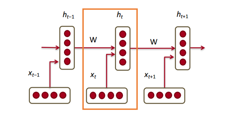
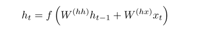
The hidden state in each module of the RNN is a function of both the word vector and the hidden state vector at the previous time step.

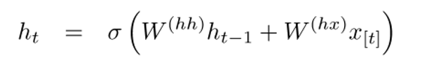
If you take a close look at the superscripts, you’ll see that there’s a weight matrix W^hx which we’re going to multiply with our input, and there’s a recurrent weight matrix W^hh which is multiplied with the hidden state vector at the previous time step. Keep in mind that these recurrent weight matrices are the same across all time steps. This is the key point of RNNs. Thinking about this carefully, it’s very different from a traditional 2 layer NN for example. In that case, we normally have a distinct W matrix for each layer (W1 and W2). Here, the recurrent weight matrix is the same through the network.

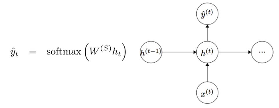
To get the output (Yhat) of a particular module, this will be h times W^S, which is another weight matrix.

Let’s take a step back now and understand what the advantages of an RNN are. The most distinct difference from a traditional NN is that an RNN takes in a sequence of inputs (words in our case). You can contrast this to a typical CNN where you’d have just a singular image as input. With an RNN, however, the input can be anywhere from a short sentence to a 5 paragraph essay. Additionally, the order of inputs in this sequence can largely affect how the weight matrices and hidden state vectors change during training. The hidden states, after training, will hopefully capture the information from the past (the previous time steps).

Gated Recurrent Units (GRUs)

                Let’s now look at a gated recurrent unit, or GRU. The purpose of this unit is to provide a more complex way of computing our hidden state vectors in RNNs. This approach will allow us to keep information that capture long distance dependencies.  Let’s imagine why long term dependencies would be a problem in the traditional RNN setup. During backpropagation, the error will flow through the RNN, going from the latest time step to the earliest one. If the initial gradient is a small number (say < 0.25), then by the 3^rd or 4^th module, the gradient will have practically vanished (chain rule multiplies gradients together) and thus the hidden states of the earlier time steps won’t get updated.

In a traditional RNN, the hidden state vector is computed through this formulation.

The GRU provides a different way of computing this hidden state vector h(t). The computation is broken up into 3 components, an update gate, a reset gate, and a new memory container. The two gates are both functions of the input word vector and the hidden state at the previous time step.

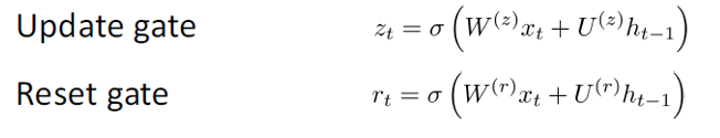
The key difference is that different weights are used for each gate. This is indicated by the differing superscripts. The update gate uses W^z and U^z while the reset gate uses W^r and U^r.

Now, the new memory container is computed through the following.

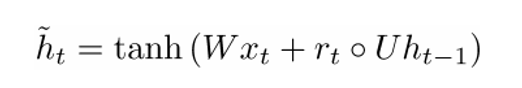
(The open dot indicates a Hadamard product)

Now, if you take a closer look at the formulation, you’ll see that if the reset gate unit is close to 0, then that whole term becomes 0 as well, thus ignoring the information in h_t-1 from the previous time steps. In this scenario, the unit is only a function of the new word vector x_t.

The final formulation of h(t) is written as

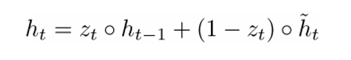
h_t is a function of all 3 components: the reset gate, the update gate, and the memory container. The best way to understand this is by visualizing what happens when z_t is close to 1 and when it is close to 0. When z_t is close to 1, the new hidden state vector h_t is mostly dependent on the previous hidden state and we ignore the current memory container because (1-z_t) goes to 0. When z_t is close to 0, the new hidden state vector h_t is mostly dependent on the current memory container and we ignore the previous hidden state. An intuitive way of looking at these 3 components can be summarized through the following.

• Update Gate:
  • If z_t ~ 1, then h_t completely ignores the current word vector and just copies over the previous hidden state (If this doesn’t make sense, look at the h_t equation and take note of what happens to the 1 - z_t term when z_t ~ 1).
  • If z_t ~ 0, then h_t completely ignores the hidden state at the previous time step and is dependent on the new memory container.
  • This gate lets the model control how much of the information in the previous hidden state should influence the current hidden state.
• Reset Gate:
  • If r_t ~ 1, then the memory container keeps the info from the previous hidden state.
  • If r_t ~ 0, then the memory container ignores the previous hidden state.
  • This gate lets the model drop information if that info is irrelevant in the future.
• Memory Container: Dependent on the reset gate.

A common example to illustrate the effectiveness of GRUs is the following. Let’s say you have the following passage.

and the associated question “What is the sum of the 2 numbers?”. Since the middle sentence has absolutely no impact on the question at hand, the reset and update gates will allow the network to “forget” the middle sentence in some sense, and learn that only specific information (numbers in this case) should modify the hidden state.

Long Short Term Memory Units (LSTMs)

                If you’re comfortable with GRUs, then LSTMs won’t be too far of a leap forward. An LSTM is also made up of a series of gates.

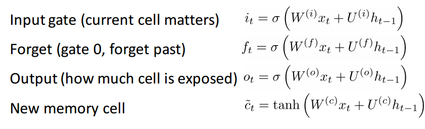
Definitely a lot more information to take in. Since this can be thought of as an extension to the idea behind a GRU, I won’t go too far into the analysis, but for a more in depth walkthrough of each gate and each piece of computation, check out Chris Olah’s amazingly well written blog post. It is by far, the most popular tutorial on LSTMs, and will definitely help those of you looking for more intuition as to why and how these units work so well.

Comparing and Contrasting LSTMs and GRUs

                Let’s start off with the similarities. Both of these units have the special function of being able to keep long term dependencies between words in a sequence. Long term dependencies refer to situations where two words or phrases may occur at very different time steps, but the relationship between them is still critical to solving the end goal. LSTMs and GRUs are able to capture these dependencies through gates that can ignore or keep certain information in the sequence. 

The difference between the two units lies in the number of gates that they have (GRU – 2, LSTM – 3). This affects the number of nonlinearities the input passes through and ultimately affects the overall computation. The GRU also doesn’t have the same memory cell (c_t) that the LSTM has.

Before Getting Into the Papers

                Just want to make one quick note. There are a couple other deep models that are useful in NLP. Recursive neural networks and CNNs for NLP are sometimes used in practice, but aren’t as prevalent as RNNs, which really are the backbone behind most deep learning NLP systems.

Alright. Now that we have a good understanding of deep learning in relation to NLP, let’s look at some papers. Since there are numerous different problem areas within NLP (from machine translation to question answering), there are a number of papers that we could look into, but here are 3 that I found to be particularly insightful. 2016 had some great advancements in NLP, but let’s first start with one from 2015.

Memory Networks

Introduction

                The first paper, we’re going to talk about is a quite influential publication in the subfield of Question Answering. Authored by Jason Weston, Sumit Chopra, and Antoine Bordes, this paper introduced a class of models called memory networks.

The intuitive idea is that in order to accurately answer a question regarding a piece of text, you need to somehow store the initial information given to you. If I were to ask you the question “What does RNN stand for”, (assuming you’ve read this post fully J) you’ll be able to give me an answer because the information you absorbed by reading the first part of this post was stored somewhere in your memory. You just had to take a few seconds to locate that info and articulate it in words. Now, I have no clue how the brain is able to do that, but the idea of having a storage place for this information still remains.

The memory network described in the paper is unique because it has an associative memory that it is able to read and write to. It’s interesting to note that we don’t have this type of memory with CNNs or with Q-Networks (for reinforcement learning) or with traditional neural nets. This is in part because the task of question answering relies so heavily upon being able to model or keep track of long-term dependencies, such as keeping track of the characters in a story or a timeline of events. With CNNs and Q-Networks, “memory” is sort of built into the weights of the network as it learns different filters or mappings from states to actions. At first look, RNNs and LSTMs could be used, but these typically aren’t able to remember or memorize inputs from the past (which in question answering is quite critical).

Network Architecture

                Okay, so now let’s look at how this network processes the initial text it is given. Like with most machine learning algorithms, the first step is to convert the input into a feature representation. This could entail using word vectors, part of speech labeling, parsing, etc. It’s really just up to the programmer.

The next step would be taking the feature representation I(x) and allowing our memory m to be updated to reflect the new input x we’ve received.

You can consider the memory m to be a sort of an array that is made up of individual memories m_i. Each of these individual memories m_i can be a function of the memory m as a whole, the feature representation I(x), and/or itself. This function G can be as simple as just storing the whole representation I(x) in the individual memory unit m_i.  You can modify this function G to update past memories based on new input.  The 3^rd and 4^th steps involve reading from memory, based on the question, to get a feature representation o, and then decoding it to output a final answer r.

The function R could be an RNN that is used to convert the feature representations from memory into a readable and accurate answer to the question.

Now, let’s look at step 3 a little closer. We want this O module to output a feature representation that would best match a possible answer to our given question x. Now this question is going to be compared to every single individual memory unit and is going to be “scored” based on how well the memory unit supports the question.

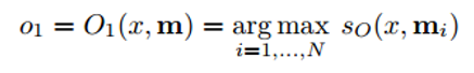
We take the argmax of the scoring function to find the output representation that best supports the question (You can also take multiple of the highest scoring units, doesn’t have to be limited to 1). The scoring function is one that computes the matrix product between different embeddings of the question and the chosen memory unit[s] (check paper for more details). You can think of this as when you multiply the word vectors of two words in order to find their similarity. This output representation o is then fed into an RNN or LSTM or another scoring function which will output a readable answer.

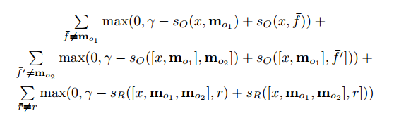
This network is trained in a supervised manner where training data includes the original text, the question, supporting sentences, and the ground truth answer. Here is the objective function.

For those interested, these are some papers that built off of this memory network approach

• End to End Memory Networks (only requires supervision on outputs, not supporting sentences)
• Dynamic Memory Networks
• Dynamic Coattention Networks (Just got released 2 months ago and had the highest test score on Stanford’s Question Answering Dataset at the time)

Tree LSTMs for Sentiment Analysis

Introduction

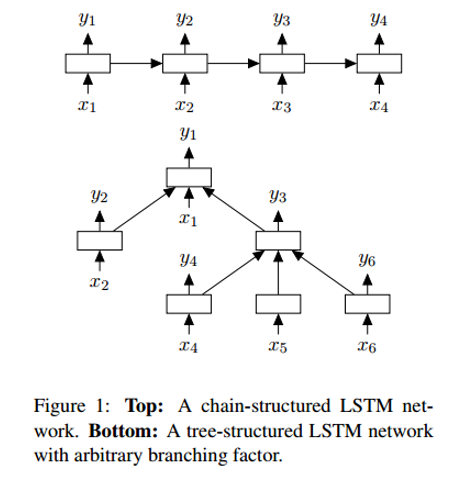
                The next paper looks into an advancement in Sentiment Analysis, the task of determining whether a phrase has a positive or negative connotation/meaning. More formally, sentiment can be defined as “a view or attitude toward a situation or event”. At the time, LSTMs were the most commonly used units in sentiment analysis networks. Authored by Kai Sheng Tai, Richard Socher, and Christopher Manning, this paper introduces a novel way of chaining together LSTMs in a non-linear structure.  

The motivation behind this non-linear arrangement lies in the notion that natural language exhibits the property that words in sequence become phrases. These phrases, depending on the order of the words, can hold different meanings from their original word components. In order to represent this characteristic, a network of LSTM units must be arranged into a tree structure where different units are affected by their children nodes.

Network Architecture

                One of the differences between a Tree-LSTM and a standard one is that the hidden state of the latter is a function of the current input and the hidden state at the previous time step. However, with a Tree-LSTM, its hidden state is a function of the current input and the hidden states of its child units.

With this new tree-based structure, there are some mathematical changes including child units having forget gates. For those interested in the details, check the paper for more info. What I would like to focus on, however, is understanding why these models work better than a linear LSTM.

With a Tree-LSTM, a single unit is able to incorporate the hidden states of all of its children nodes. This is interesting because a unit is able to value each of its children nodes differently. During training, the network could realize that a specific word (maybe the word “not” or “very” in sentiment analysis) is extremely important to the overall sentiment of the sentence. The ability to value that node higher provides a lot of flexibility to network and could improve performance.

Neural Machine Translation

Introduction

                The last paper we’ll look at today describes an approach to the task of Machine Translation. Authored by Google ML visionaries Jeff Dean, Greg Corrado, Orial Vinyals, and others, this paper introduced a machine translation system that serves as the backbone behind Google’s popular Translate service. The system reduced translation errors by an average of 60% compared to the previous production system Google used.

Traditional approaches to automated translation include variants of phrase-based matching. This approach required large amounts of linguistic domain knowledge and ultimately its design proved to be too brittle and lacked generalization ability. One of the problems with the traditional approach was that it would try to translate the input sentence piece by piece. It turns out the more effective approach (that NMT uses) is to translate the whole sentence at a time, thus allowing for a broader context and a more natural rearrangement of words.

Network Architecture

                The authors in this paper introduce a deep LSTM network that can be trained end to end with 8 encoder and decoder layers.  We can separate the system into 3 components, the encoder RNN, decoder RNN, and attention module. From a high level, the encoder works on the task on transforming the input sentence to vector representation, the decoder produces the output representation, and then the attention module tells the decoder what to focus on during the task of decoding (This is where the idea of utilizing the whole context of the sentence comes in).

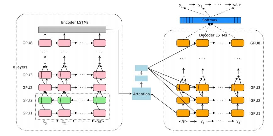
The rest of the paper mainly focuses on the challenges associated with deploying such a service at scale. Topics such as amount of computational resources, latency, and high volume deployment are discussed at length.

Conclusion

                With that, we conclude this post on how deep learning can contribute to natural language processing tasks. In my mind, some future goals in the field could be to improve customer service chatbots, perfect machine translation, and hopefully get question answering systems to obtain a deeper understanding of unstructured or lengthy pieces of text (like Wikipedia pages).

 Special thanks to Richard Socher and the staff behind Stanford CS 224D. Great slides (most of the images are attributed to their slides) and fantastic lectures.

Dueces.

Sources

Tweet